
Kepler: Part 1 - Data Acquisition
This is Part 1 of a series in which we work with data from the Kepler Space Telescope. Here, we first learn how to select our target data from the NASA Exoplanet Archive and then create a script to download the corresponding light curves from the Mikulski Archive for Space Telescopes (MAST).
Our ultimate goal is to process the data and create a machine learning model to detect potential exoplanets among the dataset. If you would like some background information as to what exoplanets and light curves are, I highly suggest reading Andrew Vanderburg’s tutorial where he provides both great explanations and animations relating to exoplanets and light curves.
Environment
If you wish to follow along, make sure you have Python installed on your system. I will be working with Python 3.6.8 on macOS 10.14.3.
Data Acquisition
Exoplanet Archive
We will work with the Kepler Q1-Q17 DR24 TCE dataset in particular because of its completeness and already existing human labels. A TCE is a threshold crossing event; these are objects that the Kepler pipeline flagged as being of interest in regards to possible exoplanets.
Once there, we are faced with a wall of rows and columns. Go to ‘Select Columns’ and enable 'Autovetter Training Set Label', found under ‘Autovetter Parameters’. Click on ‘Update’. A new column titled ‘av_training_set’ should appear at the end. By clicking and dragging the column name, move it so that it is the second column, ahead of ‘KepID’.
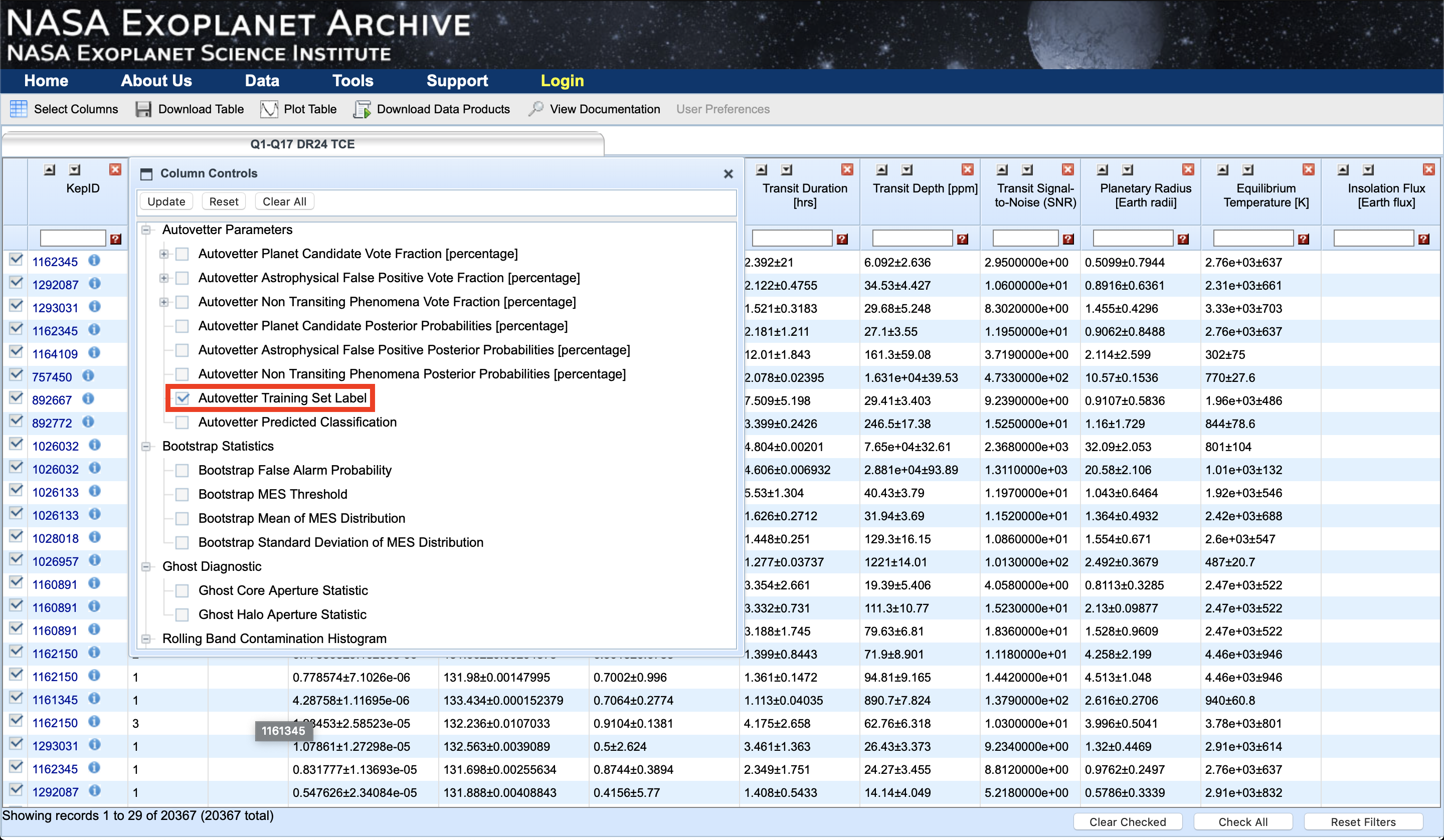
For more detail about how the training set labels are constructed, see Autovetter Planet Candidate Catalog for Q1-Q17 Data Release 24.
There are four types of labels:
- PC : Planetary Candidate
- AFP : Astrophysical False Positive
- NTP : Non-Transiting Phenomenon
- UNK : Unknown
Now would be a good time to look over the other columns to familiarize yourself with the available data.
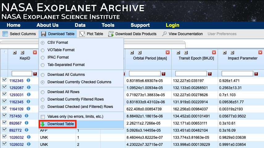
Ensure that all rows are checked and go to ‘Download Table’. If not already selected, select ‘CSV Format’ and click on the 'Download Table' button from the dropdown menu. Rename the CSV file to 'dr24_tce.csv' and store it in the directory you will be working in. In my case, my working directory will simply be named ‘kepler’.
MAST
Now that we have our CSV file containing our target objects, we can download their corresponding light curves from MAST.
Note: Doing so for all TCEs will require about 87 Gbs of space. You could repeat the steps above to acquire a smaller subset or remove objects from the downloaded CSV file.
The best option for downloading the light curves is a wget script that reads the CSV file and retrieves the light curves. You can read more about creating your own script here. So as to not distract from working with the data itself, we will refer to a python script that generates the wget scripts. This one was written by Chris Shallue. You can get the script, generate_download_script.py, from his GitHub here.
To run the script, open Terminal and navigate to your kepler directory. You can learn more about using the terminal here. My directory is located at ‘/Users/antonio/kepler’, so I will navigate there using the cd command. We then use pwd and ls to verify that our files are there. Substitute my directory for yours wherever you see mine.
Call the script
python generate_download_script.py --kepler_csv_file=dr24_tce.csv --download_dir=dataA new script was generated, which we now run
./get_kepler.sh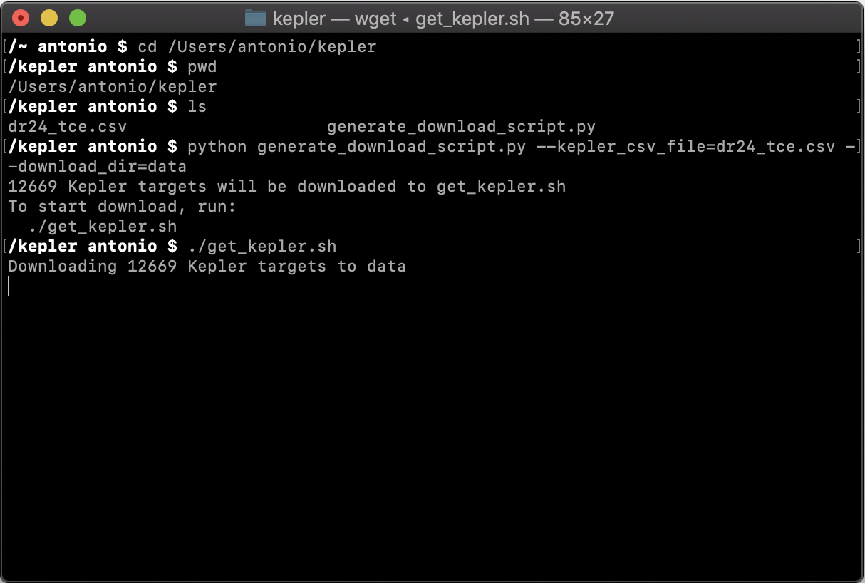
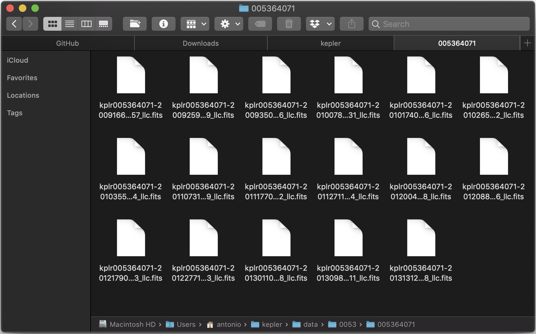
Once the script has finished downloading the light curves, there should be a new folder containing all the TCE’s light curves. That folder contains folders with four-digit names, since the TCEs have been grouped by the first four-digits of their KepID. For example, TCE 005364071 can be found in ‘/data/0053/005364071’. For every TCE there are about 15 to 18 FITS files, which contain the light curves.
Summary
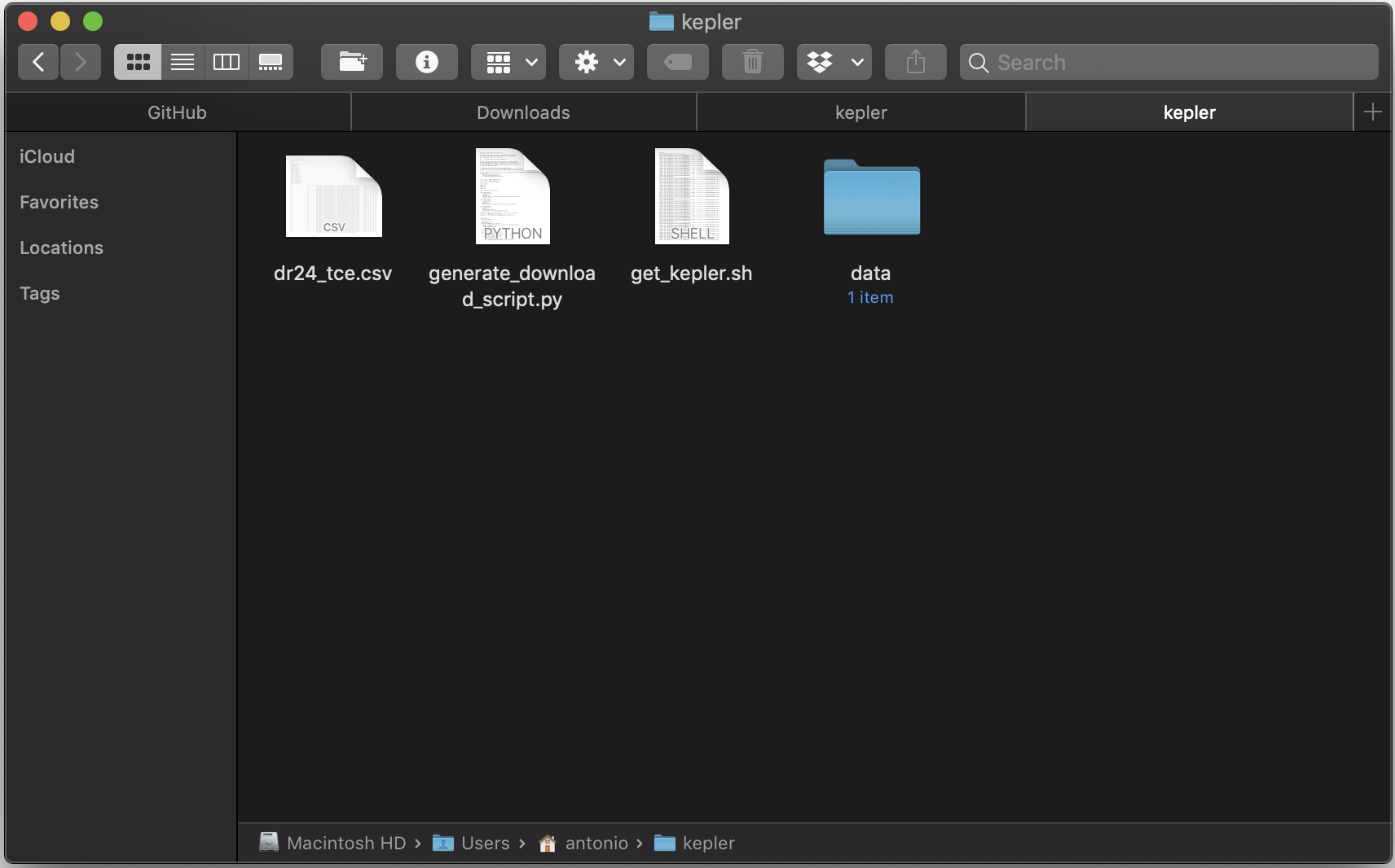
We now have a working directory that contains a CSV file with all the information about each TCE, two scripts used to download the light curves, and a folder which contains all of the corresponding light curves.
Those two scripts are no longer needed and can be removed. I will create a new folder called ‘scripts’ and move them there.
We went over how to select our target objects from the NASA Exoplanet Archive and how to use scripts to download the corresponding light curves as FITS files from MAST. Now that we have this data, we can begin analyzing and processing it. That is the topic of the next parts of this series.